Last week my advisor came back from a long trip and encouraged me to re-do my modelling of galaxy rotation curves using MCMC [Markov chain Monte Carlo] instead of a
Levenberg-Marquardt implementation I've been using.
I had dropped this line of approach before because I didn't understand why MCMC algorithms such as
Metropolis - Hastings work. It's quite difficult to find a simple, intuitive, non-Bourbaki-ish explanation of MCMC principles, and even more difficult to understand it without writing code in parallel.
MCMC is, as many things we take for granted today,
a by-product of nuclear weapons research and the Cold War. It merges
Monte Carlo methods, i.e. repeated random sampling, and
Markov chains -- a prescription for
processes which next state depends only on the current state, and is not correlated with the preceding ones.
MCMC methods are used for solving a wide variety of problems, frequently for model selection too. A crucial concept here is the
parameter space -- i.e. the set of all possible parameters one's model can have. For instance, if your model is a straight line, described by an equation
y = mx+b,
x and
y are the independent and dependent variables of your model, whereas
m and
b are the model parameters. The (
m, b) plane is your two-dimensional parameter space, representing all slope
m and intercept
b combinations a straight line can have. Here's a nice
literary explanation.
If you have any data you are trying to model at your disposal, your model becomes constrained by it: not all (
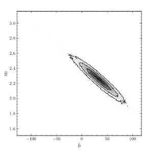
m, b) pairs describe your data equally well. There are locations at the parameter space where the model cannot describe the data by any means, let's say, the line is way above the data and goes away to infinity because the slope is wildly inadequate. There are locations that describe pretty decent models -- let's say, with a slightly wrong offset or slightly wrong slope. The goodness of model in parameter space can look similar to this picture, taken from
a pedagogical article by D. Hogg et al., here the darker, denser regions show better combinations of
m and
b:
Evaluating how well a model fits the data is a separate branch of science, but that is often helped by a quantity called
Chi-squared, or Chi2. It's simply the squared difference between your data values (
y') and the values (
y) your model predicts, divided by squared uncertainties on
y' you know from your data. This way bad datapoints do not influence your model selection much. You can think about Chi-squared as measure of distance between your model and your data -- you sure want to make it as small as possible.
The crux of MCMC model selection methods is random sampling from model parameter distribution in such a manner that the sample is proportional to the real parameter distribution -- you pick more points from denser regions in the parameter space, and just a few points from the areas with unlikely parameter combinations. What you end up with are the distributions of your model parameters, given the data -- not only a (probably local) minimum given by simple fitting, but a full distribution, from which you can estimate the uncertainties of your model, see its limitations, etc.
You probably don't need MCMC to fit a straight line to data, but if you have several parameters in your model (I've got 7 or 5) with non-trivial interrelations, your parameter space becomes high-dimensional, with a complicated landscape of better/worse fitness peaks and troughs.
So, how does MCMC work? I'll go through the Metropolis algorithm step by step. Imagine you have the straight line model
y = mx+b and some data you are trying to fit with it.
- You randomly select a pair of initial m, b values m0, b0 and calculate how good the model y = m0*x + b0 is (by calculating it's ln-likelihood, which is simply a function of Chi-squared for that model).
- You make a small random step in parameter space, obtaining a m1, b1 pair.
- Then you check if the model y = m1*x + b1 is better than the previous model, y = m0*x + b0, by looking at the ratio of their likelihoods. If this model describes the data better, you keep this pair of parameters (save it into an array) and go to step 2. If it is worse, you go to the next step.
- You draw a random number between 0 and 1 again. If the ratio of likelihoods from step 3 is lower than this number, you reject this (m1, b1) pair and go back to (m0, b0), trying step 2 again with a new random step. If it is higher, you keep (m1, b1) and repeat step 2 from this new position.
I couldn't understand this last step for quite a long time. What it does -- and why you draw a second random number -- is
selecting the less likely parameter pairs with a probability proportional to their likelihood. You still have some points in highly unlikely regions of parameter space, but not many -- because you reject most of the steps as the likelihood ratio is so low, you rarely draw a random number lower than that. Conversely, you get many more points from the denser, 'better' regions in parameter space, because the likelihood ratio is closer to 1 and you keep most of the points you draw there. This is magic for two reasons:
-- in the end you can simply draw histograms of
m and
b and see how they are distributed in the parameter space, characterise those distributions, calculate the standard deviations, see if they are multimodal (have multiple local minima), etc.. When you use the common fitting algorithms, you frequently get just a few numbers characterising (possibly local) minima, and not the full distributions of your parameters.
-- The fact that some low-likelihood points are still picked up allows exploring all the parameter space, thus you don't get stuck in a local minimum.
There's one more reason! Imagine you don't care about one or more of the parameters and only want to explore the distribution of the other ones (say, you only care about the slope). If you run MCMC, as the end result you obtain the full distribution of the parameter(s) of interest, using the entire, realistic distribution of the unimportant ones. That's called
marginalisation of the
nuisance parameters and may involve some nasty integrals otherwise.
I wrote my own MCMC code in order to understand the algorithm in detail and develop intuition, then switched to
emcee by D. Foreman-Mckey et al., which is a well-designed, parallelised, fast
code that makes life easier (and I don't have to worry about things like burn-in, initial position, autocorrelation time, thinning and step size selection too much). Here's the
scholarly article and
some highly useful wraparound scripts by Neil Crighton for setting-up and running emcee.
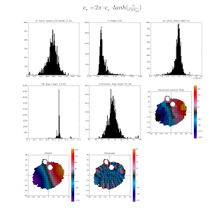
Here is what I get, fitting the stellar rotation of a galaxy (CALIFA IFU observations) with a model having 5 free parameters. Inclination and velocity amplitude (the upper left panel) are strongly coupled, and that's evident!